How can I "group by" and sum a column in excel?

Question

I'm trying to figure out how to "group by" values in an Excel spreadsheet.

Given the following example (this is an inventory sheet I use at my restaurant:)

At the far right of the spreadsheet there is a column named Cost of Goods Sold.

I would like to be able to come up with a total COGS figure for each Category.

Is this possible in excel? Moreover, I'd like to do it in a separate worksheet so that the first worksheet (what is pictured) isn't affected.

Any ideas?

Thanks!

Answer 1

The feature you want to use is Pivot Tables. It's really easy to do exactly what you want with just a few clicks once you learn how to use that feature.

Answer 2

You can also do this with the Subtotal feature.

1. Click the Data tab in Excel's ribbon toolbar
2. Click the Sort button and sort by your category column
3. Click the Subtotal button and fill in the dialog as appropriate, then click OK

For example...

At each change in: Category

Use function: Sum

Add subtotal to: Cost of Goods Sold

Answer 3

To do this with a pivot table:

1. Select all the data (including the column labels)
2. Insert > PivotTable
3. Drag a field into a dimension (row or column) of the pivot table to group by it
4. Drag a field into the "values" area to calculate a metric about it; in this case, Sum.

Answer 4

I am assuming that you are looking for the total COGS for an account like grocery for instance for week 1.

sumif is the easiest way to come up with that data. example taken from your picture:

=sumif(d2:d?,"grocery",j2:j?)

I have placed the question marks since I cannot see the whole sheet. You would select the entire column D where you have account data. D2 thru D?, Same with weekly usage column J2 thru J?.

The formula will look in the D column for the text grocery, if it is present it will add the cells in column J that correspond with D columns that have the word grocery in it. (or whatever text you put in the formula for it to look for)

Answer 5

The most trivial approach may be a Excel Sort operation followed by a Excel Subtotal operation.

It yields what you seek without changing the whole layout of your data as Pivot operation would.

Sorting

• Click the Data tab (or press Alt-A on keyboard)
• Click Sort (or press S on keyboard)
• Click the drop down arrow next to "Sort by" in the main area of popup window.
• Select "Category" since this is what you want to group by.
• Click OK!

Subtotal

Click the Data tab (or press Alt-A on keyboard)

Click Subtotal icon (or press B on keyboard)

Now that your data is sorted, read and fill the Subtotal popup like you were reading natural English:

       At each change in
          Category (Click dropdown arrow and select this)
       Use function
          Sum (Click dropdown arrow and select this)
       Add subtotal to
          Cost of Good Sold (Select the columns you wanted to total for individual categories)

   Click OK!

Answer 6

In Excel 2013 there will be a "grouping" option.

1. Select your table.
2. Go to the Data tab.
3. Click Structure > Grouping.

See screenshot below, unfortunately, it's German - but the icons will help you to find it.

Answer 7

I do this all the time with vba. I am pretty sure I have used the same method since office 95', with minor changes made for column placement. It can be done with fewer lines if you don't define the variables. It can be done faster if you have a lot of lines to go through or more things that you need to define your group with.

I have run into situations where a 'group' is based on 2-5 cells. This example only looks at one column, but it can be expanded easily if anyone takes the time to play with it.

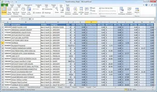
This assumes 3 columns, and you have to sort by the group_values column. Before you run the macro, select the first cell you want to compare in the group_values column.

'group_values, some_number, empty_columnToHoldSubtotals
'(stuff goes here)
'cookie  1   empty
'cookie  3   empty
'cake    4   empty
'hat     0   empty
'hat     3   empty
'...
'stop

Sub subtotal()
  ' define two strings and a subtotal counter thingy
  Dim thisOne, thatOne As String
  Dim subCount As Double

  ' seed the values
  thisOne = ActiveCell.Value
  thatOne = ActiveCell.Offset(1, 0)
  subCount = 0

  ' setup a loop that will go until it reaches a stop value
  While (ActiveCell.Value &lt&gt "stop")

    ' compares a cell value to the cell beneath it.
    If (thisOne = thatOne) Then
      ' if the cells are equal, the line count is added to the subcount
      subCount = subCount + ActiveCell.Offset(0, 1).Value

    Else
      ' if the cells are not equal, the subcount is written, and subtotal reset.
      ActiveCell.Offset(0, 2).Value = ActiveCell.Offset(0, 1).Value + subCount
      subCount = 0

    End If

    ' select the next cell down
    ActiveCell.Offset(1, 0).Select

    ' assign the values of the active cell and the one below it to the variables
    thisOne = ActiveCell.Value
    thatOne = ActiveCell.Offset(1, 0)
  Wend

End Sub

Answer 8

As another method, which does not trump the pivot table, can use the Filter formula on tabular data, e.g. for the following:

Col1	Col2
1	1
2	1
3	2
4	2
5	3
6	4

Adding a column with the formula

=SUM(FILTER([Col1], [@Col2]=[Col2], 0))

will provide the following table

Col1	Col2	Col3
1	1	3
2	1	3
3	2	7
4	2	7
5	3	5
6	4	6

which Col3 is the sum of Col1 grouped by Col2.

Could use a Unique() to grab the grouped values in separate cells instead of inserting another column in the table, and combine this with a BYCOL(array, LAMBDA(x, fn)) which makes the solution more dynamic.

If the solution exists elsewhere please throw the link in the comments :)

Answer 9

1) Select range of data.
2) Copy range to clipboard.
3) Open new data base Access.
4) Design new Table or Paste Range.
5) Create View, SQL View.
6) Create Query "SELECT cell, SUM(data)AS Total FROM Table GROUP BY cell".

Answer 10

In Excel 2013:

-Click Data

-Click Subtotal